Random Settings in Cellular Automata Machines

In cellular automata machines such as the CAM8 and SIMP/STEP (which is CAM8’s software incarnation) memory is organized into planes: each plane represents a certain type of information. A single cell spans through planes.

Consider, for example, the HPP (Hardy, de Pazzis and Pomeau) lattice gas model. In HPP, gas particles travel along the lines of a square grid and collide in the nodes of the grid. The collision rule states that, if exactly two particle meet in a node, and they come from opposite direction, then they bounce with a angle; in all other cases, particles go straight ahead. In SIMP/STEP, we can construct the HPP lattice gas model by defining interaction as follows:

    def hpp_rule():
        if north == south and east == west:
            north._ = east
            east._  = south
            south._ = west
            west._  = north
    hpp_step = Rule(hpp_rule)

Suppose, however, that the update rule is not deterministic but randomized. For example, in the FHP lattice gas model, which has six direction on a triangular lattice, the principle is the same as for HPP, but the direction (clockwise or counter-clockwise) of the rotation is chosen at random. This can be done by initializing a single plane with zeros and ones, and have the cell read the corresponding bit and interpret it as the direction of the rotation. To ensure non-repetition, during the update the plane will be moved by a random offset. In SIMP/STEP, it would look more or less like the following:

    def fhp_rule():
        if north == south and east == west and ne == sw:
            if r: # rotate clockwise
                north._ = west
                west._  = sw
                sw._    = south
                south._ = east
                east._  = ne
                ne._    = north
            else: # rotate counter-clockwise
                north._ = ne
                west._  = north
                sw._    = west
                south._ = sw
                east._  = south
                ne._    = east
    fhp_step = Sequence([Stir([r]), Rule(fhp_rule)])

It might be the case, however, that we need different probability distributions in different points. In such a case, it would be anti-economical to set as many random planes as needed distributions: instead, one would want to set as few planes as possible with random distributions, and exploit the flexibility given by the application of boolean functions to said planes. Different cells might then have different types, and interpret differently the state of the random planes.

Let us make a quick example with a single plane, initialized with probability . If we pass a bit, whose value is with probability , to a boolean function of a single argument, then the output bit will have a Bernoulli distribution with parameter which depends on both and . Specifically, will be 0 if is the constant function , if is the identity, if is the negation, and 1 if is the constant function 1: which exhausts the possibilities of a single bit.

In general, random bits with independent Bernoulli distrinutions of parameters can yield up to possible distributions for the output bit of an -to-1 boolean function. It then becomes of interest to understand how to set the parameters in order to obtain a convenient range of values for just by changing the specific . In particular, we are interested in obtaining the uniform range

which minimizes the maximum distance between the value desired and the one which is actually obtained. A general solution to this problem was described by Mark Smith in his 1994 PhD thesis under the supervision of Tommaso Toffoli.

Before examining Smith’s method, let us observe that the denominator in the formula above is the -th Mersenne number. The sequence of Mersenne numbers is defined by the formula

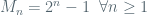
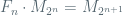
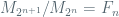
In general, Mersenne number are not primes: indeed, it is a standard exercise in elementary number theory that is a factor of if is a factor of , so that a Mersenne number can be prime only if its index is prime: such condition is not sufficient, as .

Let us go back to the case : we know that, in this case, given the value of the parameter we can get any of the values , , , . To have these values coincide with , , , it is thus sufficient to set .

Let us now consider the case . We know that, in this case, the denominator should be : so we are strongly tempted to set again, then , which would give us when is the boolean AND. But how do we know that we may get the remeining values as well?

To prove this, let’s do a thought experiment. Suppose we have a rectangle, whose height and width are in ratio: let us make two cuts, one on the short side at of the heigth, the other on the long side at of the width. The sizes of the four pieces obtained are in proportion with each other as the numbers , , , and . But every integer number between and has a unique writing as a sum of one or more of the fourn numbers above: and indeed, we can also choose the output probability with any given value of the form with an integer between and . To decide which function we have to use to get probability for the output b, we proceed as follows:

1. We write .
2. We choose so that for every .

For example, if we want , we take the function that takes value only on the pair .

To generalize to arbitrary many bits, we introduce Fermat numbers, defined by the formula

We easily get

that is, the product of the -th Fermat number and the -th Mersenne number is the -th Mersenne number. This leads us to

Theorem. If the probability of bit  is , then all and only the probabilites  with between and can be obtained. Such arrangement is the only one that allows recovering all said probabilities in output, up to a rearrangement of the bits.

That such arrangement of probabilities for the input bits allows to obtain every possible value in the range , is easily proven via a generalization of the reasoning we made for the case . Uniqueness follows inductively from the relation .